How to Calculate Crystallite Size from XRD Using the Scherrer Equation
The width of an XRD peak is not just noise — it carries quantitative information about your material. Broader peaks mean smaller crystallites, and the Scherrer equation turns that broadening into a number. This guide walks through the calculation step by step, with a worked example you can follow along with your own data.
Why XRD peaks broaden
A perfect infinite crystal gives infinitely sharp diffraction peaks. Real materials broaden them for three reasons:
- Small crystallite size — the dominant effect for nanoparticles and thin films. Finite crystallite dimensions truncate the crystal, smearing the diffraction condition.
- Microstrain — non-uniform lattice distortions widen peaks roughly as 1/tanθ.
- Instrumental broadening — the diffractometer itself (divergence slits, finite source width) adds width that has nothing to do with your sample.
The Scherrer equation isolates the size contribution. It is the standard first-pass analysis, and it is what most papers report for crystallite size.
The Scherrer equation
D = K·λ / (β·cosθ)| Symbol | Meaning | Typical value |
|---|---|---|
| D | crystallite size (Å or nm) | — |
| K | shape factor | 0.9 (spherical) — often 0.62–1.08 |
| λ | X-ray wavelength (Å) | 1.5406 (Cu Kα₁) |
| β | FWHM of the peak in radians | — |
| θ | Bragg angle (half of 2θ) | — |
Two units trips cause most errors here: β must be in radians (not degrees), and λ must be in the same length unit as the result you want.
Step-by-step calculation
Step 1 — Read the peak position 2θ
Open your XRD pattern and locate the peak of interest. Read the angle at the top of the peak (2θ). For the worked example we use 2θ = 38.18°.
Step 2 — Measure the FWHM
FWHM (full width at half maximum) is the width of the peak at half its height, in degrees:
- Draw a baseline under the peak and read the maximum intensity.
- Find the half-maximum level.
- Measure the angular distance between the two sides of the peak at that level.
For the example: FWHM = 0.42°.
Step 3 — Convert units
Bragg angle: θ = 2θ / 2 = 38.18° / 2 = 19.09°
FWHM in radians: β = 0.42° × π / 180 = 0.00733 rad
Step 4 — Plug into the equation
Using Cu Kα₁ (λ = 1.5406 Å) and K = 0.9:
D = (0.9 × 1.5406) / (0.00733 × cos 19.09°)
  = 1.3865 / (0.00733 × 0.9449)
  = 1.3865 / 0.006926
  = 200.2 Å
  = 20.0 nm
The crystallite size is 20.0 nm.
Try it yourself: use the interactive Scherrer calculator — enter 2θ and FWHM and get D instantly.
When the simple calculation is not enough
The Scherrer result is an apparent crystallite size. Three situations demand more care:
Instrumental broadening. If your peaks are only slightly broader than a standard sample (e.g. LaB₆ or NIST 660a), the instrument contributes significantly. Correct with β²_corrected = β²_measured − β²_instrumental, or run a full profile analysis.
Microstrain. Strain broadens peaks as 1/tanθ while size broadens as 1/cosθ — the two scale differently with angle. Plot βcosθ against sinθ (Williamson–Hall plot): the intercept gives size, the slope gives strain. This needs two or more peaks.
Overlapping peaks. Partially merged peaks inflate FWHM. Fit the peaks individually (Gaussian/Lorentzian/mixed) rather than measuring the merged envelope.
Common mistakes
- Forgetting to convert FWHM to radians — the most common error; it changes the result by a factor of 57.3.
- Using the wrong K value without saying so — report which shape factor you used.
- Ignoring instrumental broadening for sharp peaks — for crystallites above ~100 nm the apparent size saturates around the instrument resolution.
- Mixing up degrees and radians for θ — cosθ is nearly flat below 20°, so this hides itself; the error grows at high angles.
- Applying Scherrer to one peak only — reporting a single value is fine, but reporting the average over several peaks (e.g. the three strongest) is much more defensible.
Do it in one click
If you would rather not measure FWHM by hand, Spectra Studio detects peak positions and FWHM automatically, computes the crystallite size for every peak (Scherrer), and with two or more peaks draws the Williamson–Hall plot with strain and R² automatically — free to download, no Python required.
Related Posts
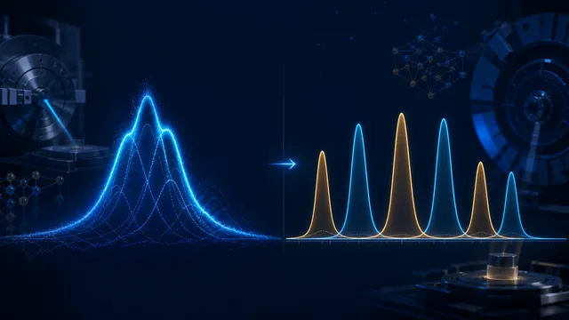
Overlapping XRD Peaks: When Manual FWHM Fails
Learn why overlapping peaks, sloping backgrounds, and instrument broadening can make manual XRD FWHM unreliable, and what to check before fitting.
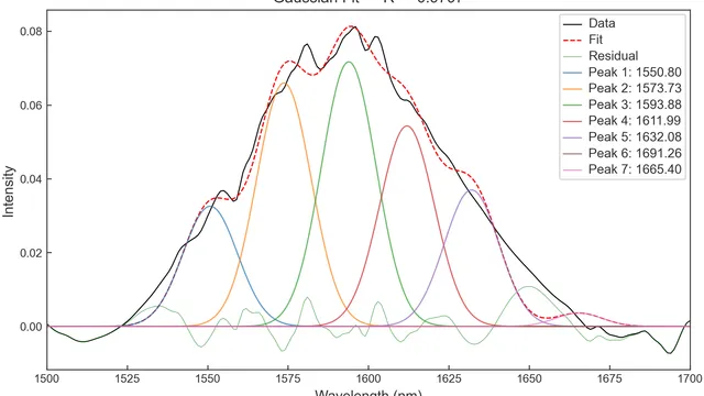
How to Fit XRD Peaks: Gaussian, Lorentzian and FWHM Analysis
A practical guide to XRD peak fitting with Gaussian, Lorentzian and mixed profiles, including FWHM, R², residuals and overlapping-peak analysis.
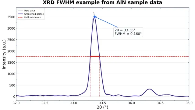
How to Calculate Crystallite Size from XRD: Scherrer and Williamson–Hall
Learn how to calculate crystallite size from XRD peak broadening with the Scherrer equation and Williamson–Hall analysis, including FWHM conversion and practical software workflow.