How to Fit XRD Peaks: Gaussian, Lorentzian and FWHM Analysis

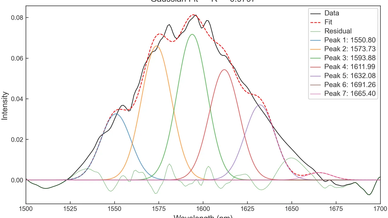
Why should you fit an XRD peak instead of reading the highest point?

Peak position, peak height, area and width are often used to discuss phase composition, crystallinity, crystallite size and treatment effects. But a simple cursor measurement becomes subjective when two reflections overlap, the background slopes, or the peak is asymmetric.

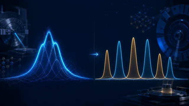
XRD peak fitting solves part of this problem by representing the measured pattern with mathematical peak profiles. A fit can separate overlapping peaks and provide a repeatable estimate of each peak’s center, FWHM and area, together with diagnostics that show how well the model follows the data.

For researchers preparing numerical tables or supplementary information, fitting is often easier to document and reproduce than measuring each width by hand.

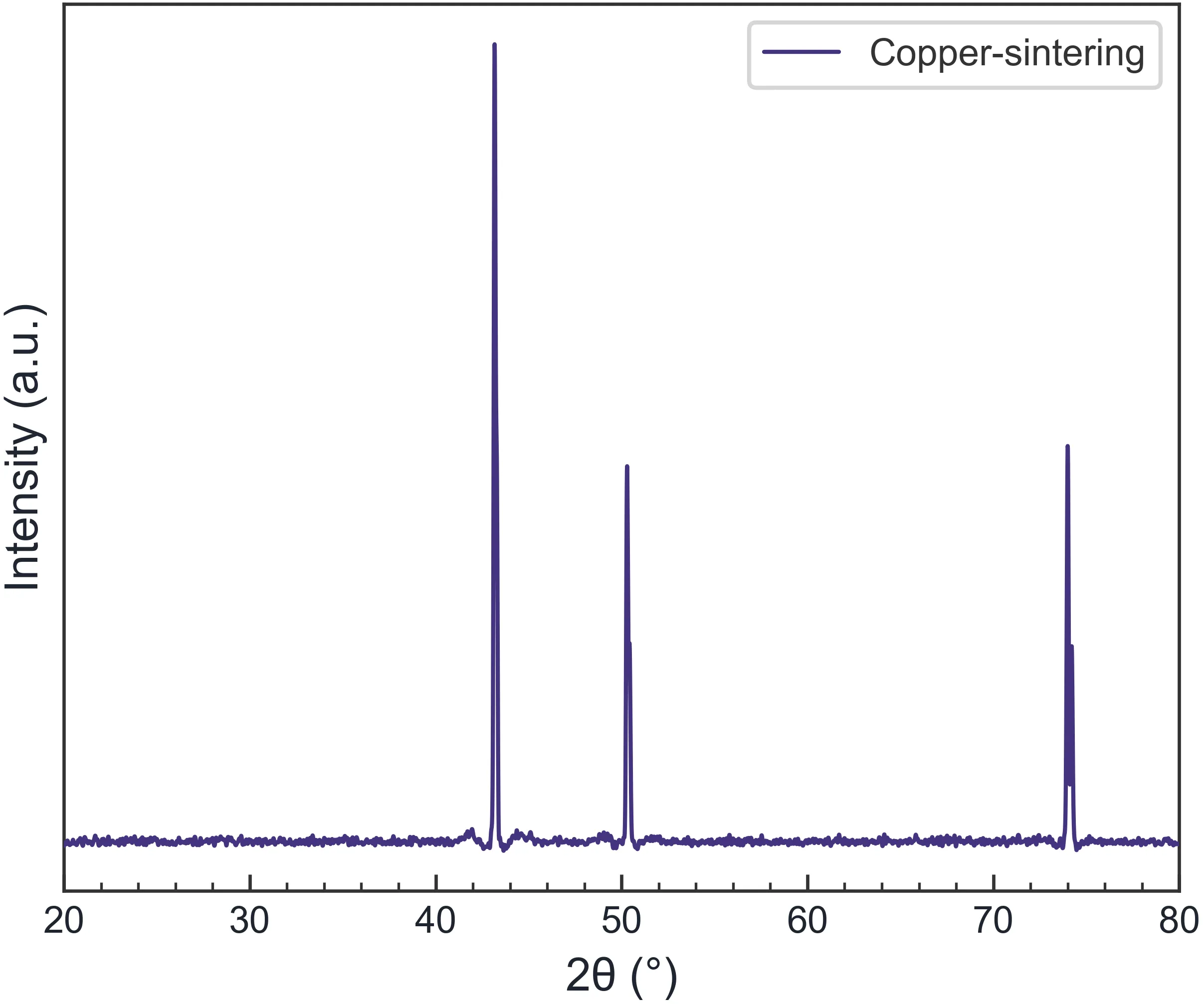
Gaussian, Lorentzian and mixed profiles

The most common profile choices include Gaussian and Lorentzian functions:

• Gaussian profile: a smooth bell-shaped profile that is often useful when broadening has a strong statistical component.
• Lorentzian profile: a profile with longer tails, used in situations where the physical or instrumental broadening is better represented that way.
• Mixed profile: a combination of Gaussian and Lorentzian contributions for peaks that are not described well by one ideal shape.

There is no single profile that is correct for every material and instrument. Select a model using the instrument context, established practice for the material, residual behavior and fit stability. Do not choose a profile only because it produces the highest R².

What should an XRD peak-fitting result contain?

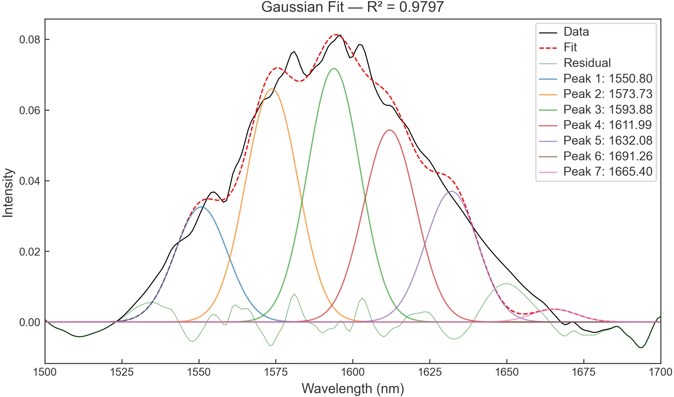
A useful fitting result normally reports:

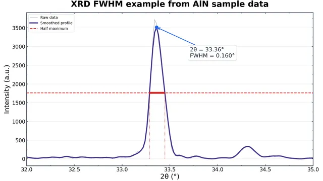
1. Peak position: the center of the reflection, such as its 2θ value.
2. FWHM: full width at half maximum, useful for comparing broadening or calculating apparent crystallite size.
3. Peak area: the integrated contribution of the fitted peak under the selected model.
4. R²: one indicator of how much variation is explained by the fit.
5. Residuals: the difference between the measured data and the fitted curve.

A high R² does not prove that the model is physically correct. Always inspect the original pattern, the total fit, each component peak and the residuals. A systematic residual pattern near a peak top or tail may indicate that the background, number of peaks or profile choice needs revision.

A practical workflow from overlapping peaks to a results table

Step 1: Load the original XRD data

Keep an untouched copy of the raw file. Spectra Studio can load PANalytical .xrdml, Bruker .brml, .uxd, and common .txt, .xy, .csv and .dat files. Direct loading reduces the chance of losing metadata or changing values during a separate conversion step.

Step 2: Treat the background carefully

Use baseline correction when the background slopes or fluorescence is obvious. If the signal is noisy, preview Savitzky–Golay smoothing before detection. Check that the smoothing window does not flatten narrow peaks, widen a feature or create an apparent peak.

A useful rule is: use processing to make detection and fitting more stable, but keep the raw data and record the processing settings.

Step 3: Detect candidate peaks automatically

Run automatic peak detection based on height and shape, then adjust the sensitivity. Return to the plot and check whether real peaks were found, background fluctuations were rejected, and an apparent broad feature should actually be split into two components.

Step 4: Fit the peaks

Spectra Studio Pro supports Gaussian, Lorentzian and mixed profiles. Detection results provide starting values, after which the fitting routine adjusts the peak position, width and intensity. The interface shows the total fitted curve, individual components and residuals together.

Step 5: Inspect the model, not just one number

Ask the following questions:

• Are the fitted positions physically plausible?
• Does the total curve follow both the peak top and the tails?
• Do the residuals show a systematic pattern?
• Is the number of peaks too small, forcing separate reflections into one envelope?
• Is the number of peaks too large, creating overfitting without physical meaning?
• Could instrumental broadening or baseline treatment be dominating the FWHM?

The final table reports position, FWHM, area, R² and residual information that can be organized into a manuscript or supplementary table.

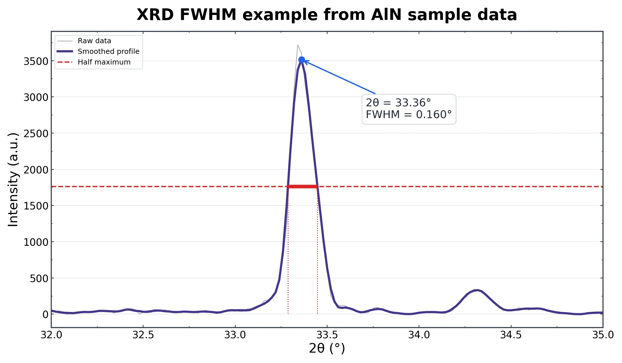
How peak fitting affects crystallite-size analysis

Peak fitting is not only a way to make a figure look smoother. When reflections overlap, separating the components gives you a more defensible single-peak FWHM before applying the Scherrer equation or a Williamson–Hall analysis.

However, a fitted width is still a model-dependent quantity. It does not mean that every part of the broadening comes from crystallite size. If you report a crystallite size, state the shape factor, X-ray wavelength and whether instrumental broadening was corrected. Changing the profile or baseline can change the calculated size.

Use Spectra Studio instead of building a fitting environment

Origin can fit several peaks, and Python can provide extensive control with packages such as scipy or lmfit. Those approaches are valuable when you need custom models, but they also require environment setup, initial-value management, file parsing and plotting code.

Spectra Studio is designed for the common laboratory workflow:

• No Python runtime or extra dependencies to install
• Multiple instrument and text formats in one loader
• Automatic detection values available as fitting starts
• Gaussian, Lorentzian and mixed profiles in one interface
• Total curve, individual components and residuals visible together
• Pro tools for Scherrer, Williamson–Hall, phase matching and Miller-index labels
• Nature, ACS and Elsevier styles with adjustable fonts, axes, lines and legends

The Free edition covers loading, smoothing, baseline correction, peak detection and watermark-free PNG/JPG export. Peak fitting and advanced quantitative analysis are unlocked in Pro. Local processing means spectra remain on the machine during analysis.

Common questions

Must every XRD peak use a Gaussian profile?

No. Gaussian, Lorentzian and mixed profiles are different models. Choose based on the material, instrument and residual behavior, then document the choice.

Does a higher R² always mean a better result?

No. R² should be evaluated together with residuals, peak count, profile choice and physical meaning. Adding unnecessary peaks can increase R² while producing an overfit.

Can I use the FWHM of an overlapping envelope?

A single FWHM measured from a strongly overlapping envelope can be misleading. Fit the components with a justified multi-peak model and inspect whether the individual widths are stable.

Is there free XRD peak-fitting software?

Spectra Studio offers a Windows Free edition for basic pattern processing and detection. Pro adds Gaussian, Lorentzian and mixed-profile fitting plus the reported fit diagnostics.

Final takeaway

The value of XRD peak fitting is not simply a smoother-looking line. It turns overlapping reflections, FWHM, peak areas and fit quality into results that can be inspected and repeated. Preserve the raw pattern, choose a defensible background and profile, check residuals, and use the fitted widths only within the limits of the model.

👉 Try Spectra Studio without Origin or Python: Open the Spectra Studio feature guide