Spectra Studio: Turn XRD, FTIR, Raman & UV-Vis Data Into Publication-Ready Figures — Without Origin or Python
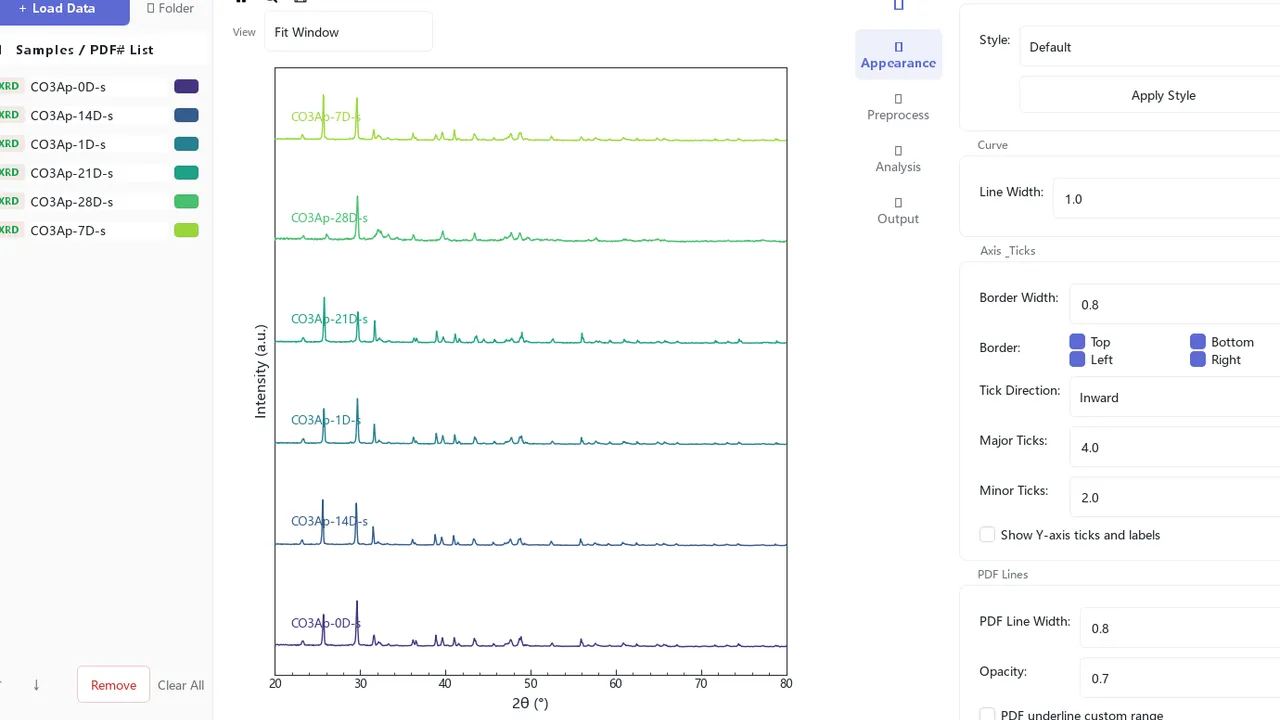
Turn XRD, FTIR, Raman & UV-Vis Data Into Publication-Ready Figures —
Without Origin or Python.
A free Windows app that reads your instrument files, cleans them, fits the peaks and exports journal-style figures. No watermark. No coding. No subscription.
Why upgrade? Pro is a one-time $79 key for peak fitting, reviewer-ready crystallite-size numbers and vector export. No subscription.
The part nobody budgets for
The science is not the slow part. The handoff is.
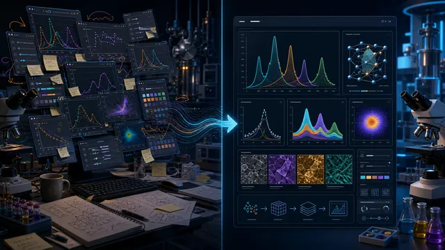
Stretch the baseline in Excel. Guess the peak width. Screenshot the result into Word. Repeat it for the next sample, then redo it when a reviewer asks for the vector figure.
Spectra Studio keeps that routine in one local workflow. Free covers the everyday figure; Pro starts when you need fitted peaks, reviewer numbers or submission-ready vector export.
See what Pro removes →The pipeline, in one line
.xlsx / .csv / .xy / .txt
fit · analyze · style
PNG · PDF · SVG · EPS · TIFF
Gallery: What Comes Out
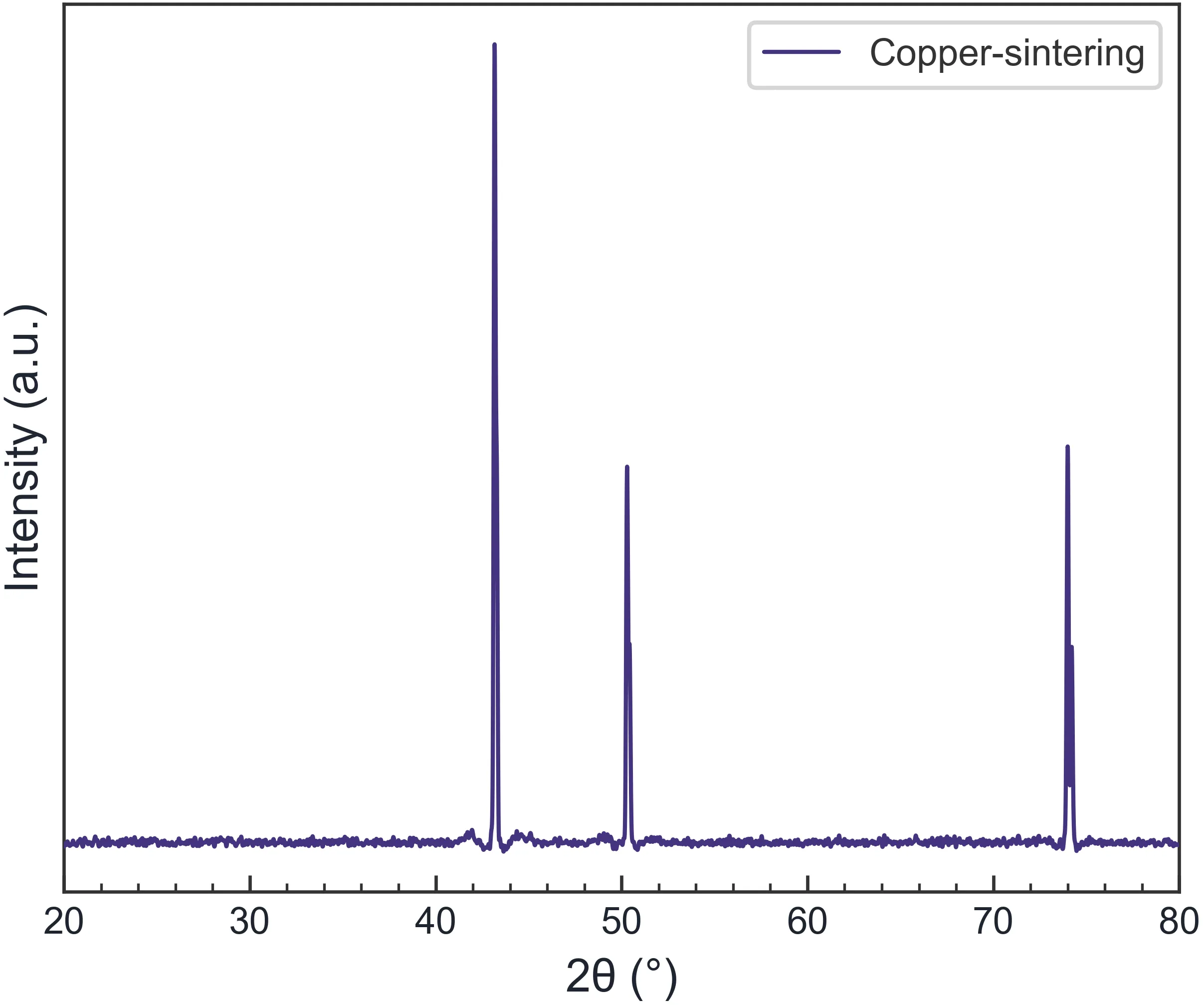
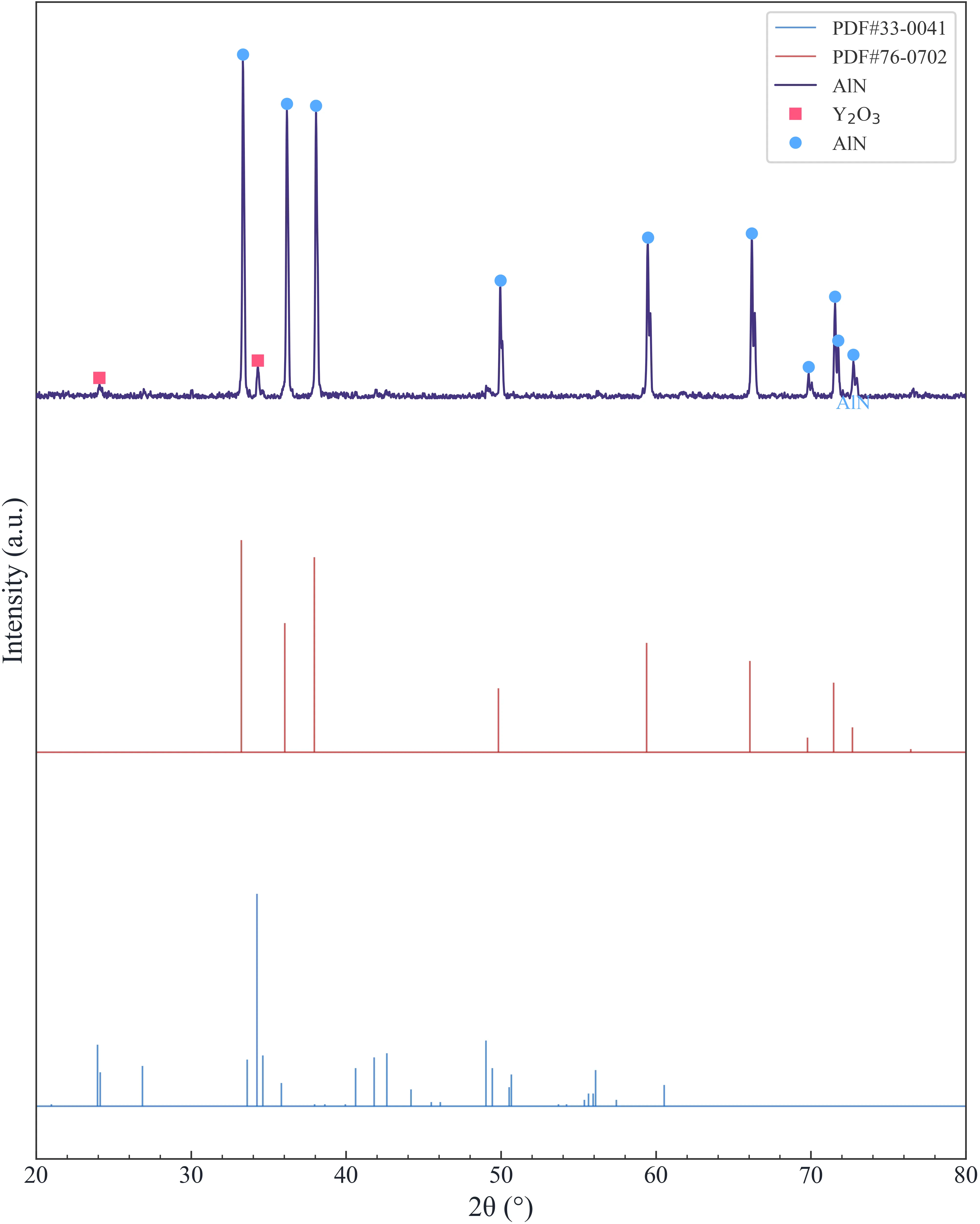
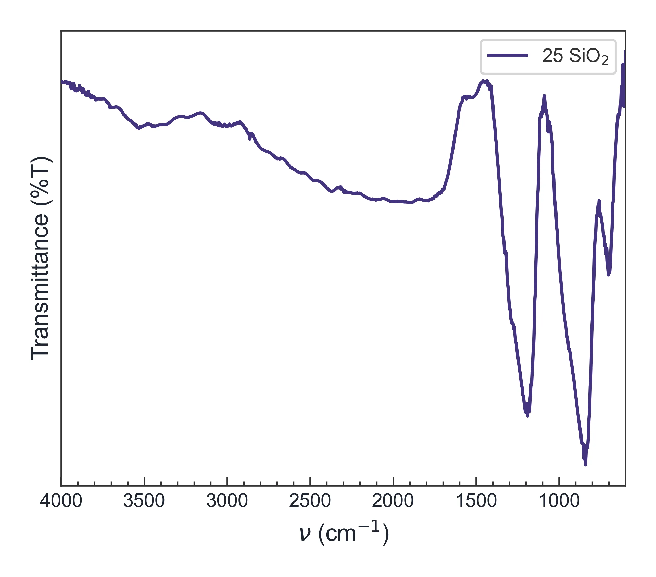
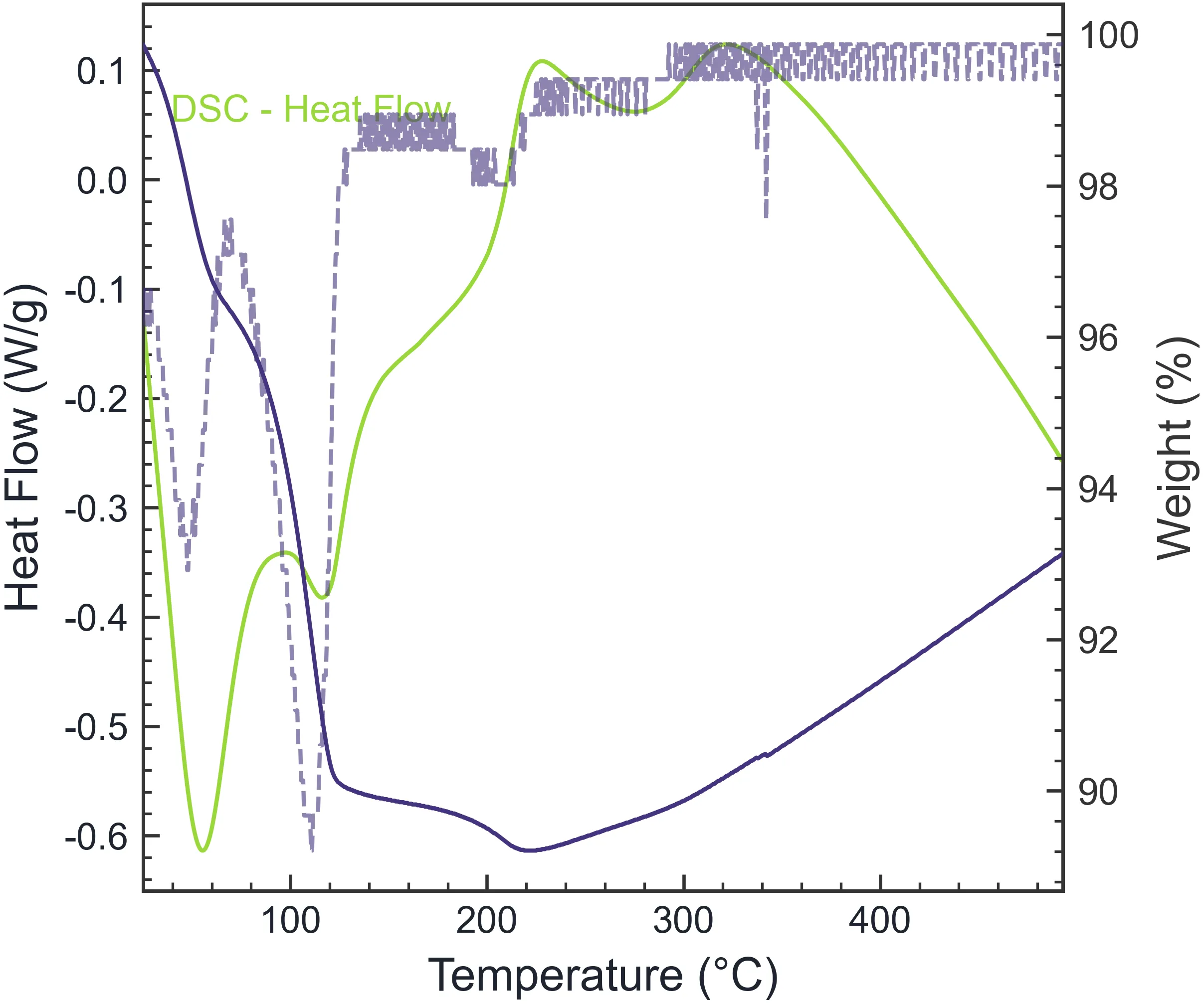
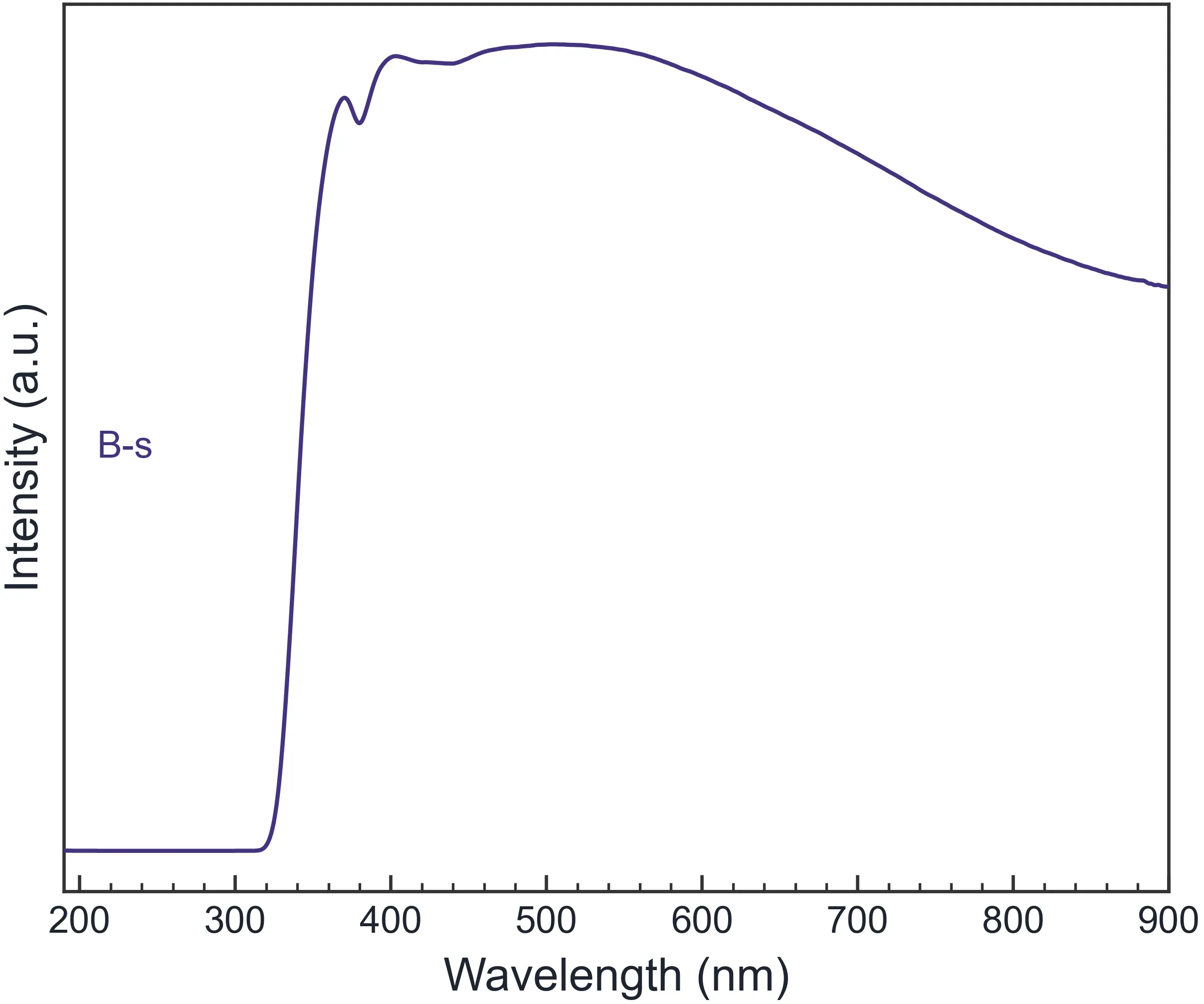
Ten finished outputs from the supplied sample folder, arranged as a responsive collage:
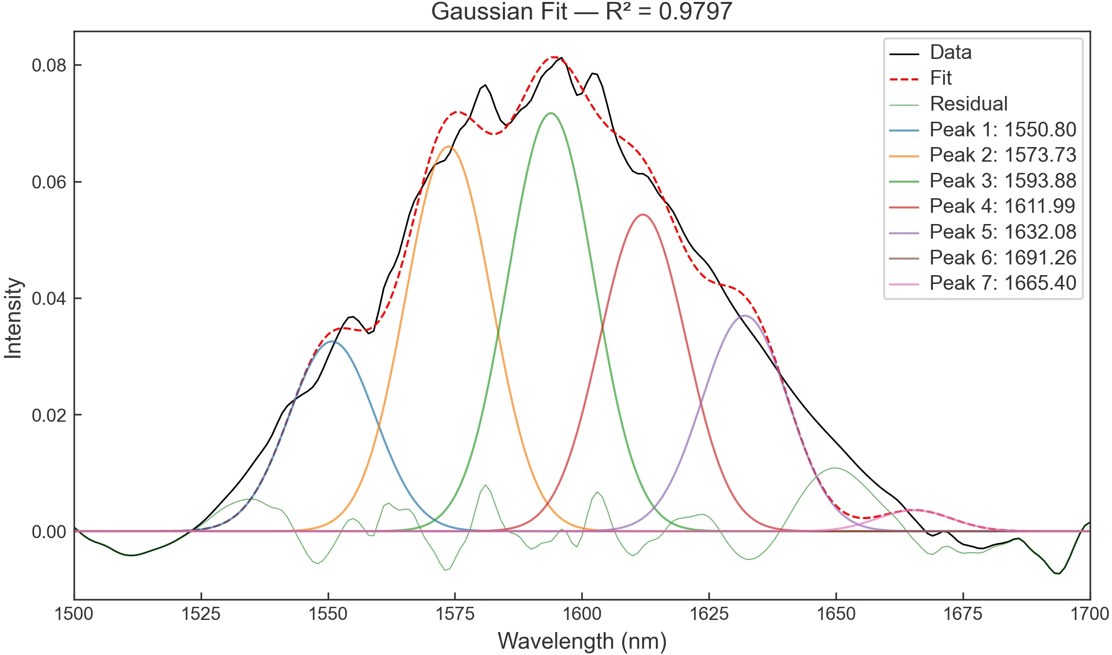
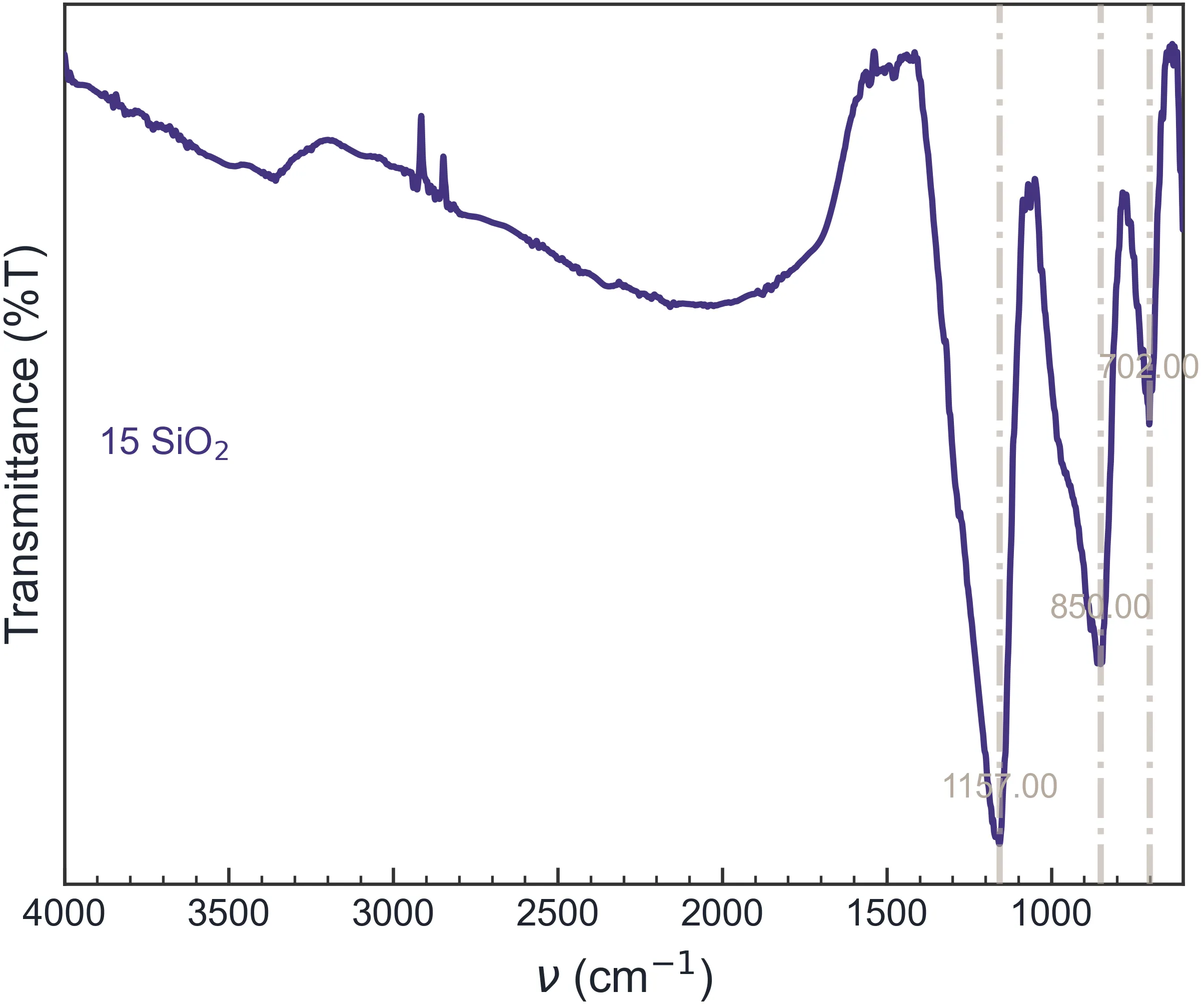
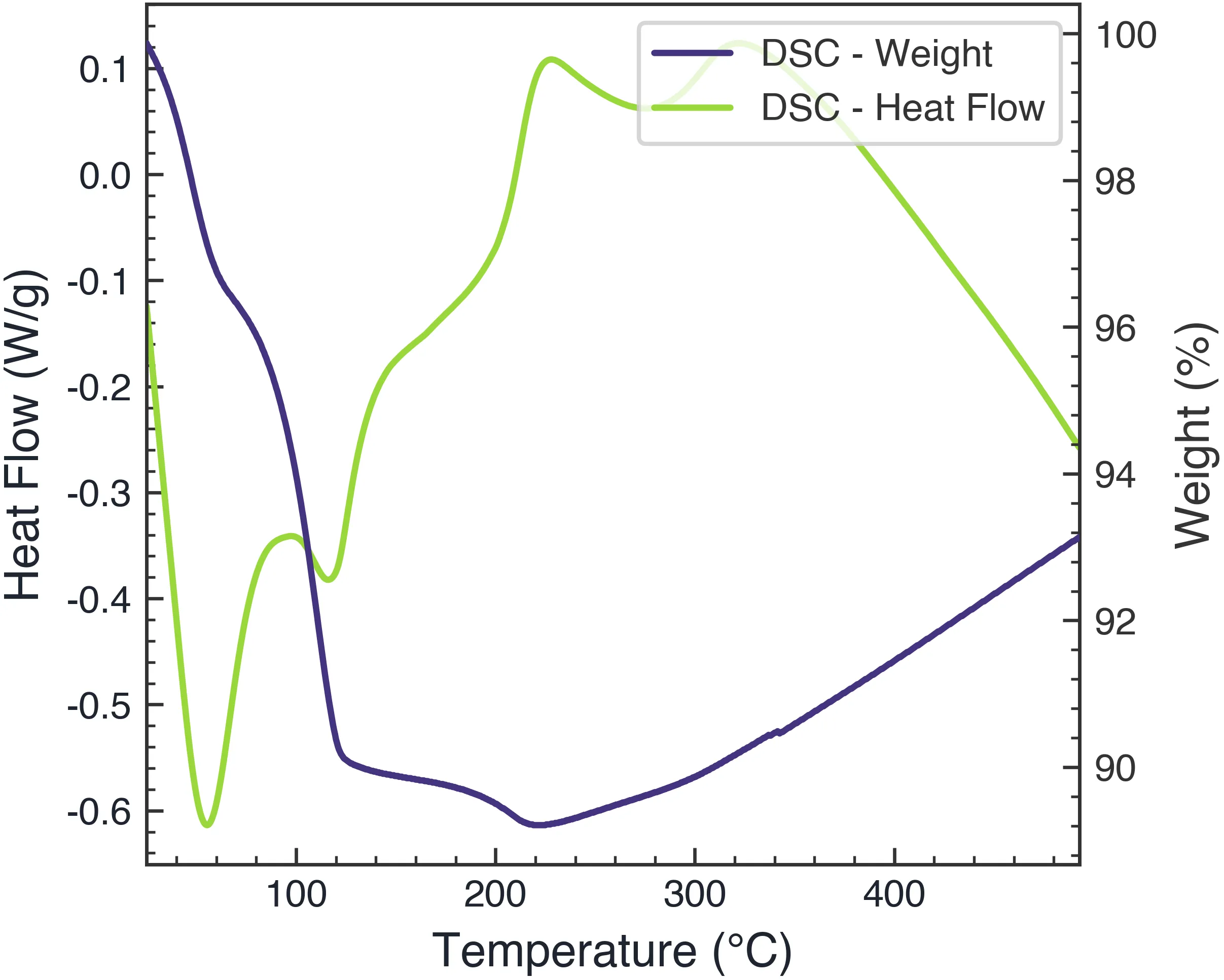
View the remaining four outputs
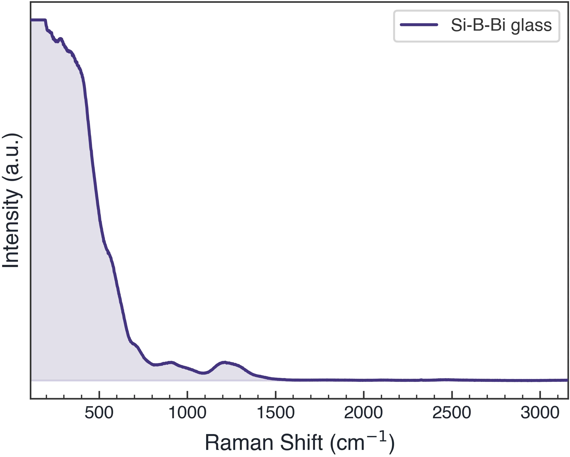
See the evidence before you decide
The gallery above uses real exports from the supplied sample folder. The live clips below show the four Pro steps, so you can judge the output before buying.
🎬 Demo: 30 seconds
What You Get in the Free Download
The installer is the complete application — all Free-edition features work immediately ($0, forever, no watermarks). Pro features are already inside the same installer; a key unlocks them in seconds, with no re-download.
- Data loading: instrument files read directly — PANalytical (.xrdml), Bruker (.brml), .uxd — plus .txt / .xy / .csv / .dat, FTIR (.asc), UV-Vis (nm, auto-detected), DSC/TGA (Excel .xlsx / .xls)
- Multi-sample management: overlay, stack, normalize, vertical offset, batch coloring
- Preprocessing: Savitzky-Golay smoothing, ALS baseline correction — every change previews live
- Peak analysis: automatic peak detection (height/shape based, sensitivity adjustable)
- Journal styles: one-click Nature / ACS / Elsevier, fine-tunable legend and ticks
- Export: PNG / JPG up to 300 DPI, watermark-free — free to use in papers and reports
Why Researchers Upgrade to Pro
These are the steps that eat your evenings — and the ones Pro compresses into seconds. Four of them, live:
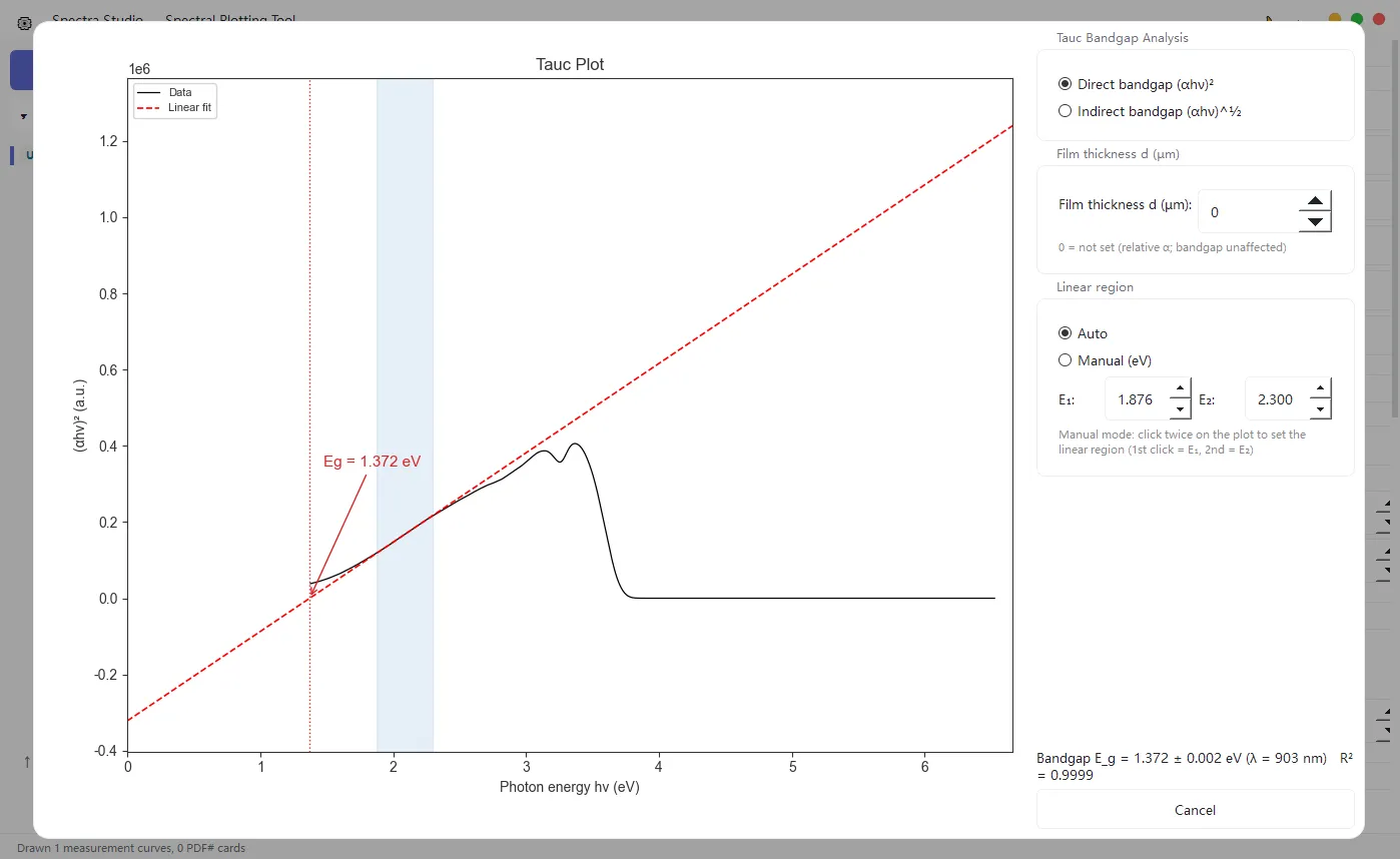
Also in Pro — Tauc bandgap (UV-Vis): load absorbance data, click “Tauc Bandgap”, and get the direct (αhν)² or indirect (αhν)^½ gap with the linear region detected automatically — Eg and its wavelength are annotated right on the plot (auto precision ≈ ±0.1 eV). Optional film thickness converts to α = 2.303A/d; leave it blank and the bandgap value is unaffected.
💡 The workflow people actually run: load → smooth/baseline → auto-detect peaks → fit → Scherrer / Williamson–Hall → Miller-index the phases → export vector. In Origin or a Python script this is an afternoon; in Spectra Studio it’s the natural order of the UI.
Full workflow, if you want the detail
Open the six-step walkthrough
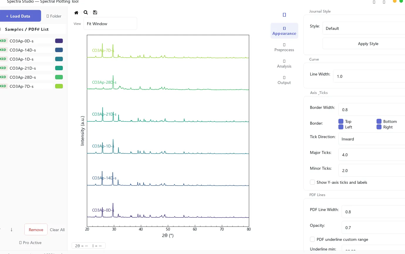
Here is the full workflow, using “six CO3Ap (carbonate apatite) XRD samples → an ACS-style submission figure” as the example.
Step 1: Load Your Data
Click “Load data” and pick files (or drag & drop them into the window). Multiple files load at once — the sample list on the left fills in and the curves appear immediately. Stack, normalize and vertical-offset options keep multi-sample comparisons clear.
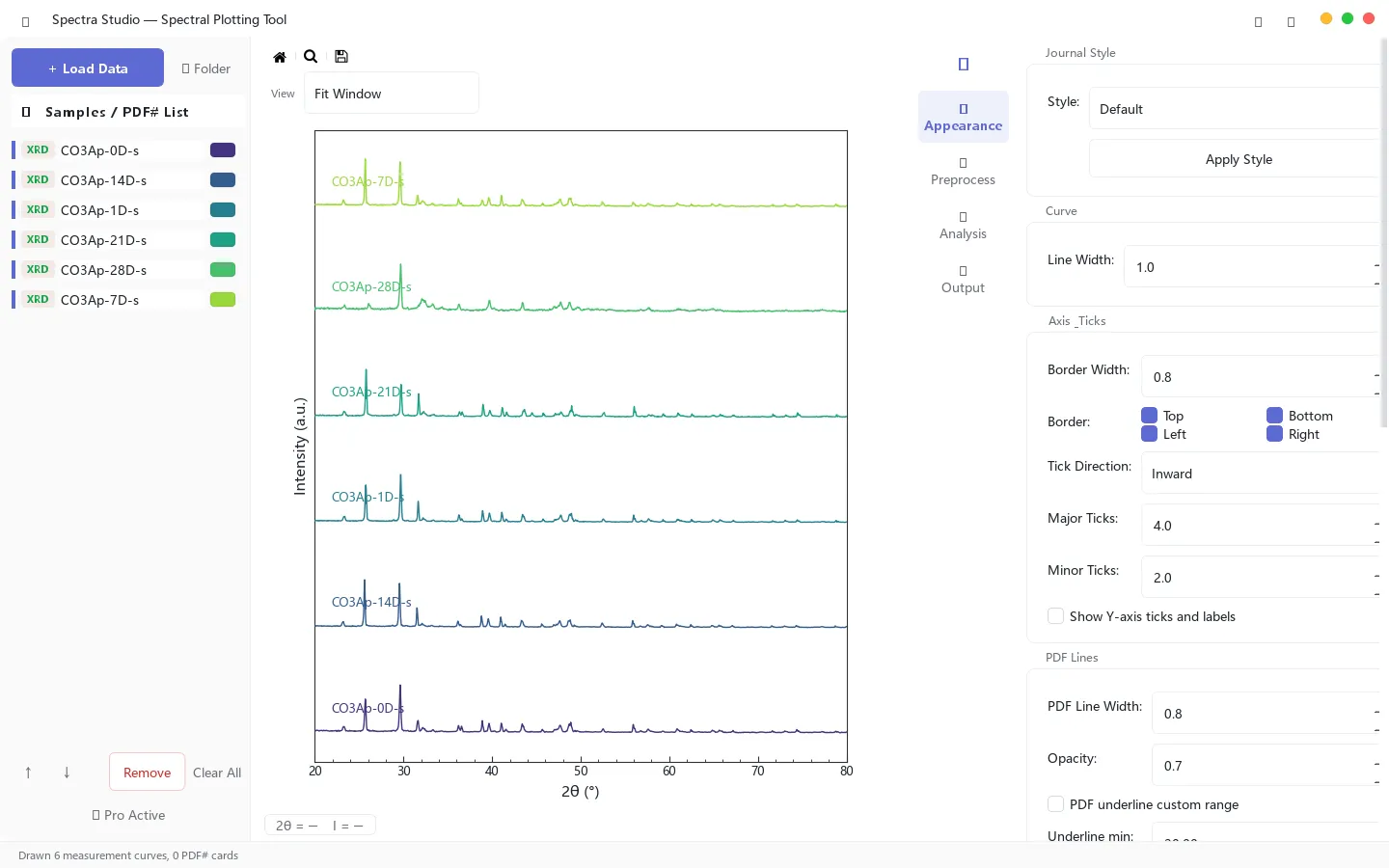
Step 2: Preprocess (Smoothing + Baseline)
Adjust the smoothing window (Savitzky-Golay) and baseline parameters (ALS) in the preprocessing panel — every change previews live. A typical workflow: smooth with a window of 9–15 to remove noise, then flatten the background with baseline correction.
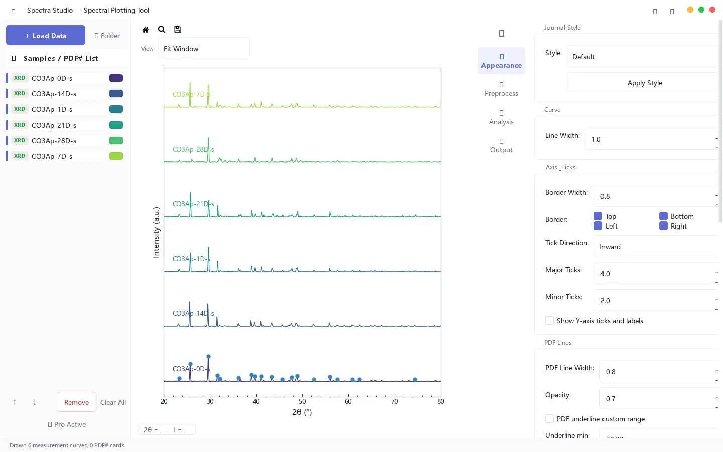
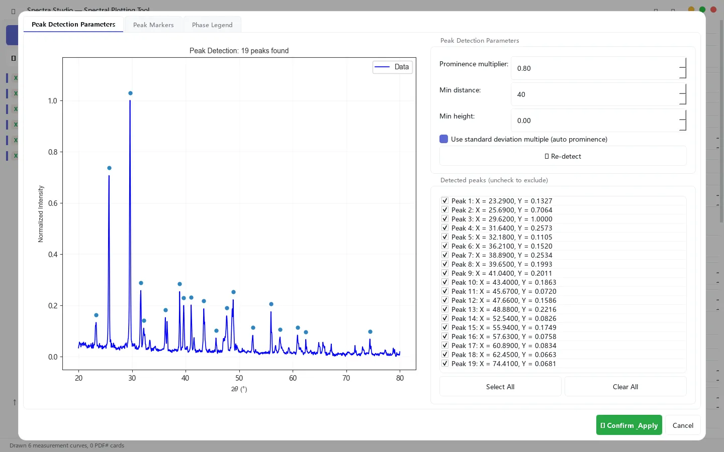
Step 3: Automatic Peak Detection
Click “Auto peak detection” and the tool marks candidate peaks based on height and shape (sensitivity is adjustable). Detected peaks appear in a table and are annotated on the plot for immediate review.
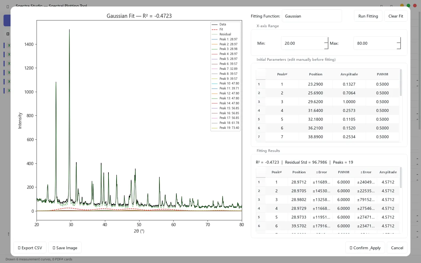
Step 4: Peak Fitting (Pro)
For overlapping peaks, use peak fitting: the tool seeds initial values from the detection results and fits Gaussian / Lorentzian (or mixed) profiles, reporting each peak’s position, FWHM, area, R² and residuals — a results table you can paste straight into supplementary materials.
Step 5: Apply a Journal Style
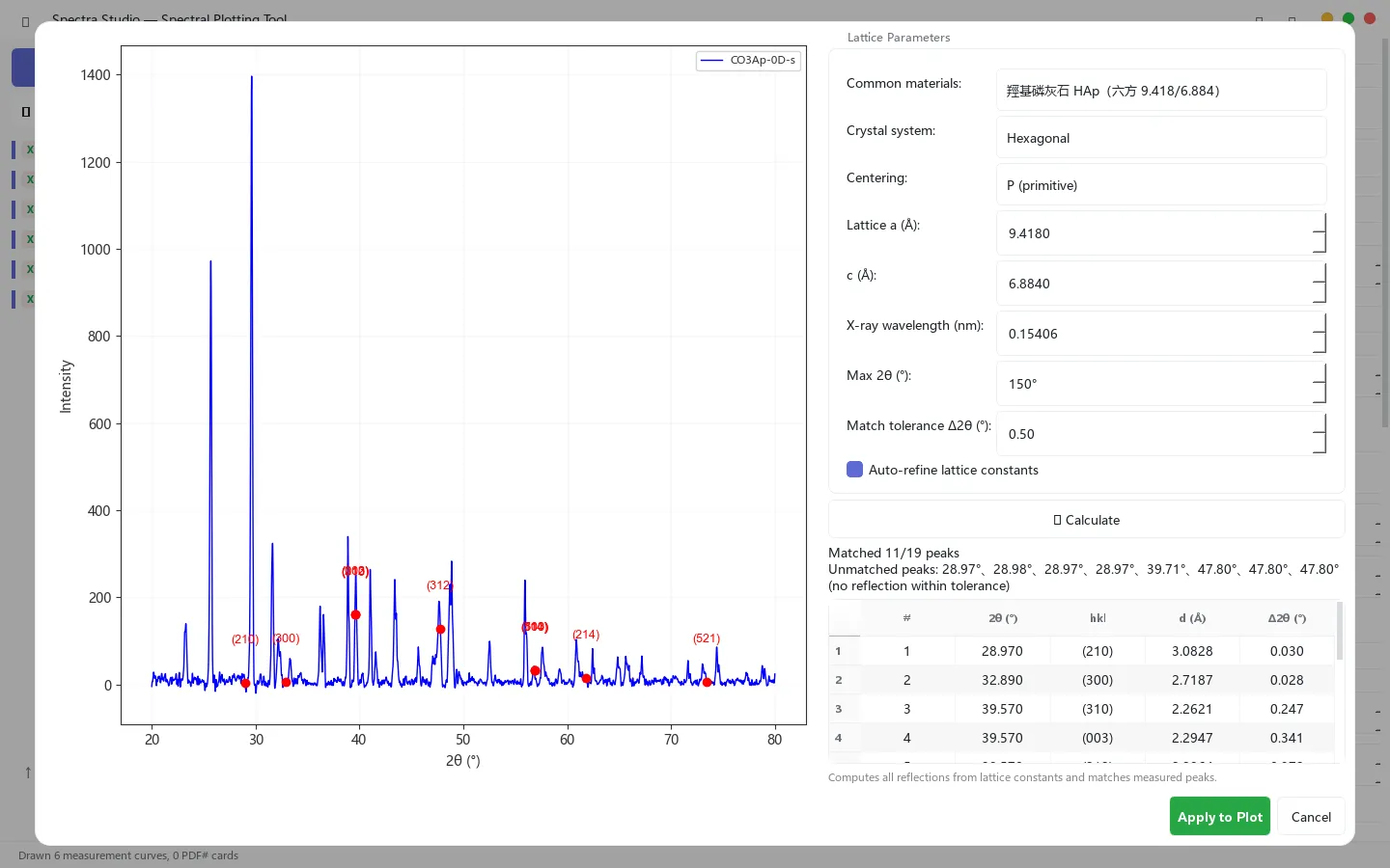
Switch between Nature / ACS / Elsevier styles with one click; legend position, fonts, line widths and tick directions are all fine-tunable. Pro adds Miller-index annotation and phase-matching labels on the plot.
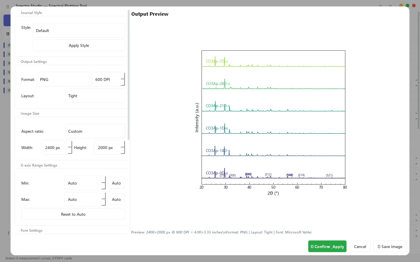
Step 6: Export
Preview before saving, then pick a format and resolution. PNG / JPG go up to 300 DPI; Pro unlocks PDF / SVG / EPS / TIFF vector export and higher resolutions — submission figures leave from here.
Crystallite Size (Pro): Grain Size, Crystallinity & Tauc Bandgap
The three quantities reviewers ask for most often — crystallite size, crystallinity and bandgap — are now computed in one click (v2.1), no more manual Excel or Origin work.
Crystallite Size & Strain (Scherrer / Williamson-Hall)
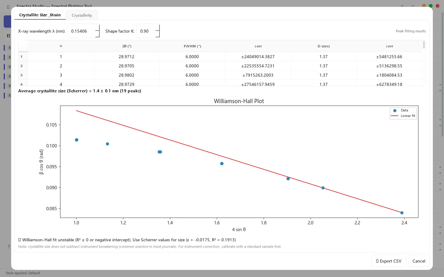
Since v2.1.1, peak fitting is no longer required first — peak sources degrade automatically: ①peak-fitting results → ②auto-detected peaks → ③one-click detection inside the dialog. You can also run peak fitting (Step 4) first, then click “Crystallite Size”. It will:
- Computes the crystallite size of every fitted peak via the Scherrer equation D = Kλ/(βcosθ), with error propagation, in a single results table
New to the calculation? Read how to calculate crystallite size from XRD or try the interactive Scherrer calculator — then come back and let the software do it in one click.
- With 2+ peaks, automatically draws a Williamson-Hall plot (βcosθ vs 4sinθ); the weighted linear fit reports crystallite size D, microstrain ε and R² — the size-vs-strain distinction reviewers love to ask about, answered in 30 seconds
- X-ray wavelength (default Cu Kα = 0.15406 nm) and shape factor K are both adjustable
Note: instrument broadening is not subtracted (common practice in most journals); for instrument correction, calibrate with a standard sample first.
Crystallinity
After fitting, the crystallinity tab of Crystallite Size computes crystallinity = fitted peak area / total area in the fit range, with the integration range drawn on the plot. Works directly for samples with a flat background; for large amorphous humps (e.g. polymers), apply baseline correction first.
Tauc Bandgap Analysis (UV-Vis)
v2.1 adds UV-Vis spectra support (wavelength in nm, auto-detected). Load absorbance data and click “Tauc Bandgap”:
- Direct (αhν)² / indirect (αhν)^½ bandgap — one-click switch
- Linear region detected automatically and a tangent drawn — Eg and its wavelength are annotated right on the plot (auto precision ≈ ±0.1 eV)
- Optional film thickness d (µm) converts to absorption coefficient α = 2.303A/d; leave blank to use relative α — the bandgap value is unaffected
- Switch to manual mode to fine-tune the linear region by clicking twice on the plot (1st click = start, 2nd = end), with instant recomputation
Technical reference
Open supported formats, analysis, styles and export details
Supported Data Formats
| Instrument / type | Formats | Notes |
|---|---|---|
| PANalytical (X’Pert etc.) | .xrdml | XML scan data read directly — no export roundtrip |
| Bruker (DIFFRAC etc.) | .brml | XML scan data read directly — no export roundtrip |
| Generic instruments | .uxd | two-column text (2θ–intensity) |
| XRD powder diffraction | .txt / .xy / .csv / .dat | 2θ–intensity columns auto-detected |
| FTIR | .asc | wavenumber axis direction auto-corrected |
| RAMAN | .txt / .xy / .csv | same loading flow as XRD |
| UV-Vis absorption | .txt / .xy / .csv | wavelength in nm auto-detected (190–1200 nm), for Tauc bandgap analysis |
| DSC / TGA | .xlsx / .xls | read Excel sheets directly |
| PDF# reference cards | built-in format | used for phase matching (Pro) |
Peak Analysis
- Auto peak detection: height/shape-based detector with adjustable sensitivity
- Peak fitting (Pro): Gaussian / Lorentzian / mixed profiles; automatic initial values (seeded from detection); outputs position, FWHM, area, R², residuals; results table exportable
- Crystallite size (Pro): Scherrer crystallite size, Williamson-Hall strain, crystallinity, Tauc bandgap (see section above)
- Calculus (Pro): first derivative (inflection/phase-transition points) and integration (area/crystallinity)
Phase Matching (Pro)
Sample peaks are matched against PDF reference cards, with the corresponding phase and Miller indices (hkl) annotated directly on the peaks, including a tolerance setting. “Is this the α phase or the β phase?” — answered in seconds.
Journal Styles
| Style | Character |
|---|---|
| Nature | borderless, minimal, compact fonts |
| ACS | left/bottom axes, bold lines, in-figure legend |
| Elsevier | full box frame, classic academic layout |
Every style remains fine-tunable: fonts, sizes, line widths, tick direction/length, legend position, axis ranges, titles.
Export Formats
| Format | Free | Pro |
|---|---|---|
| PNG / JPG | ✅ (≤300 DPI) | ✅ (up to 600 DPI) |
| PDF / SVG / EPS | — | ✅ (vector, ideal for submission) |
| TIFF | — | ✅ (300/600 DPI presets) |
Free vs. Pro
Spectra Studio comes in two editions only: Free and Pro — both live in the same installer. Download once and use the free edition immediately: no time limits, no watermarks. When you are ready, buying a key unlocks Pro in seconds — nothing to re-download.
One license. All Pro features included. Peak fitting, crystallite size, Williamson–Hall, crystallinity, Tauc bandgap, phase matching, Miller indices, vector export — every Pro feature unlocks with a single key. No tiers, no add-ons, no monthly fees.
Pro pays for itself in the hours it gives back: the evenings spent stretching baselines in Excel, guessing peak widths, and screenshotting figures into Word are exactly what Pro removes. On the night before submission, vector figures at 600 DPI go straight from the app into your manuscript — no re-drawing.
| Free | Pro | |
|---|---|---|
| Price | $0 (forever) | $79 (one-time) |
| Data loading & multi-sample management | ✅ | ✅ |
| Smoothing, baseline correction, peak detection | ✅ | ✅ |
| Journal styles & PNG/JPG export (≤300 DPI) | ✅ | ✅ |
| Peak fitting (with R² and residuals) | — | ✅ |
| Crystallite size: Scherrer / Williamson-Hall / crystallinity | — | ✅ |
| Tauc bandgap analysis (UV-Vis) | — | ✅ |
| Phase matching & Miller indices | — | ✅ |
| Vector export: PDF / SVG / EPS / TIFF (≤600 DPI) | — | ✅ |
| Watermarks / time limits | none | none |
🛒 Get Pro: Buy on Polar ($79, one-time) — pay once, receive the key immediately, and paste it into the app. One license covers all Pro features, all future updates, and works on 2 devices. Not sure? Start free, hit a Pro feature, and decide when it actually matters.
Installation & Download
- Setup program (recommended): Download SpectraStudio-Setup-v2.1.4.exe (120 MB) — double-click to install into the current user’s directory (no administrator rights needed), with a Start-menu shortcut and uninstaller.
- Portable build: Download SpectraStudio-v2.1.4-portable.exe (119 MB) — double-click to run, no installation.
- Release page: All versions on GitHub — newest versions always ship there first.
- System: Windows 10 / 11 (64-bit). The installer is about 120 MB; no Python or other runtime is required.
- Verify integrity (optional but recommended): every release page lists the SHA-256 checksum of the installer. In PowerShell:
Get-FileHash .\SpectraStudio-Setup.exe -Algorithm SHA256Compare the output against the checksum on the release page — this confirms the file you downloaded is exactly what we published.
⚠️ First launch: Windows SmartScreen may show “Windows protected your PC” for unsigned installers. Click More info → Run anyway once — we are working toward code signing so this warning disappears in future releases. (If you prefer, that’s exactly what the SHA-256 check above is for: verify, then run with confidence.)
Privacy
- 100% local processing. Spectra Studio analyzes your data on your machine; your spectra, samples and lab data never leave your computer.
- The app contains no analytics, no telemetry, no internet calls at runtime. The only network feature is the license-key check when you activate Pro.
- No account required for the Free edition — download, install, use.
FAQ
How is this different from Origin / MATLAB / Python scripts?
Origin’s licensing model is built around seats, and its scripting curve is real; Python gives you full control but demands an environment, a plotting library, and time. Spectra Studio is the middle path for the 95% case: it reads your instrument files directly, and the features you actually use in a lab — preprocessing, peak fitting, Scherrer/Williamson-Hall, Tauc, journal styling — are one click, with the exact numbers (R², residuals, ε) a reviewer will ask for. When you outgrow it, export clean data and hand it to your Python pipeline; the two coexist.
Is the Free version really free forever?
Yes. No trial countdown, no time limit, no watermark. The Free edition is a complete tool for the most common workflow (load → smooth → detect → style → export PNG). Pro only adds the deep-analysis features listed above.
Do I need to re-download the installer when I buy Pro?
No. The same installer contains both editions; a key unlocks Pro in seconds.
Is my data uploaded anywhere?
No. Everything runs locally; nothing is transmitted (see Privacy above).
Can I use the figures in my thesis/paper?
Yes — free edition included. Exported figures carry no watermark and no attribution requirement.
I use a Mac / Linux — any plan?
Windows first (the vast majority of instrument PCs run Windows). A macOS version is a possible next step; Linux users typically run it in a Windows VM or dual-boot — or use the guides below, which cover the same calculations.
Related Resources
- How to calculate crystallite size from XRD (Scherrer & Williamson–Hall, with worked examples)
- Interactive Scherrer / Williamson–Hall calculator — enter FWHM, 2θ and K, get D and ε instantly
- More guides and calculators are added continuously — all guides · all tools
Related Posts
How to Standardize Spectroscopy Figures for a Paper
Build consistent XRD, FTIR, Raman, and UV-Vis figures with repeatable offsets, fonts, axes, and export settings instead of reformatting every plot.
How to Open XRD, FTIR, Raman, and UV-Vis Files
Open common XRD, FTIR, Raman, and UV-Vis exports without a conversion maze. Learn what to verify before plotting data locally on Windows.
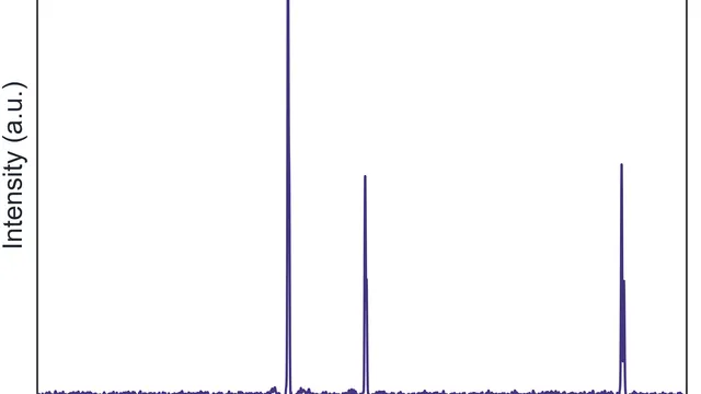
How to Make a Publication-Ready XRD Figure Without Origin
Create a clean XRD journal figure on Windows without Origin or Python: load multiple files, correct the baseline, stack samples, apply journal styles and export at 300 DPI.